Chapter 2 Spatial polygon areas
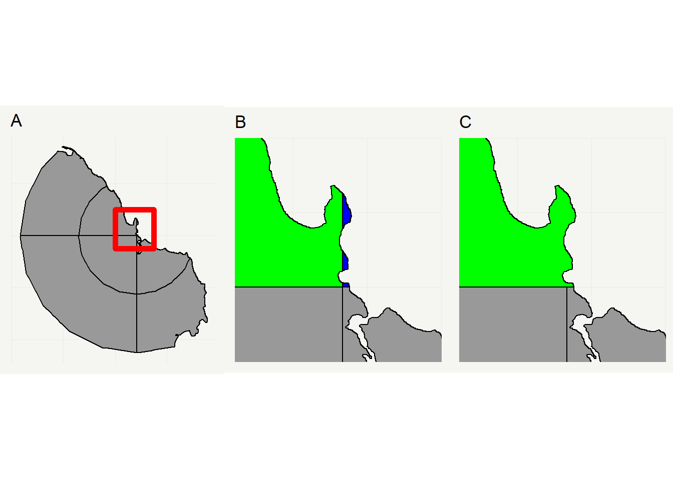 Figure 2.1: Panel A shows sampling bins for Dar es Salaam. The red rectangle is the clipped area shown in Panel B and C. The green and blue area in B are merged to the blue area in C.
First, I will discuss the urban sampling areas before turning to the more complicated border areas.
2.1 Cities
The sampling area is defined by taking a 50 km radius around the center of the respective city. The coordinates from Table 2.1 are taken from Wikipedia.1 https://Wikipedia.org
Table 2.1: Longitude and latitude of Dar es Salaam, Lusaka, and Nairobi.
| City | Longitude | Latitude |
|---|---|---|
| Dar es Salaam | 39.283333 | -6.8 |
| Lusaka | 28.283333 | -15.416667 |
| Nairobi | 36.81667 | -1.28333 |
The geosampling::prepare_sampling_bins_city function draws two circles around a point and splits both circles along the horizontal and the vertical axis in 8 pieces.
The function takes in the arguments adm0 for a variable of class SpatialPolygons, which contains the national border of the respective country, the coordinates of the respective city (coords), a variable of class SpatialPolygons, which contains lakes, and radius_inner_circle and radius_outer_circle to determine the radius of both circles.
lusaka_bins <- prepare_sampling_bins_city(
  adm0 = zambia_adm0,
  coords=city_table[2,2:3],
  lakes = lakes,
  radius_inner_circle=25,
  radius_outer_circle=50)
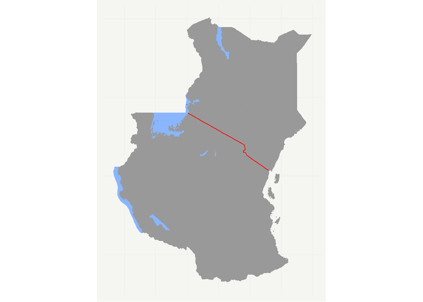 Figure 2.2: Kenya and Tanzania with shared land border in red.
Figure 2.1 shows the sampling areas for Dar Es Salaam. In Panel A Dar es Salaam has 7 different sampling areas, but one is rather small and is merged with its neighboring area (B and C).2 Map style borrowed from Timo Grossenbacher.
The sampling areas for all three cities are visualized in Figure 2.9.
2.2 Kenyan-Tanzania border
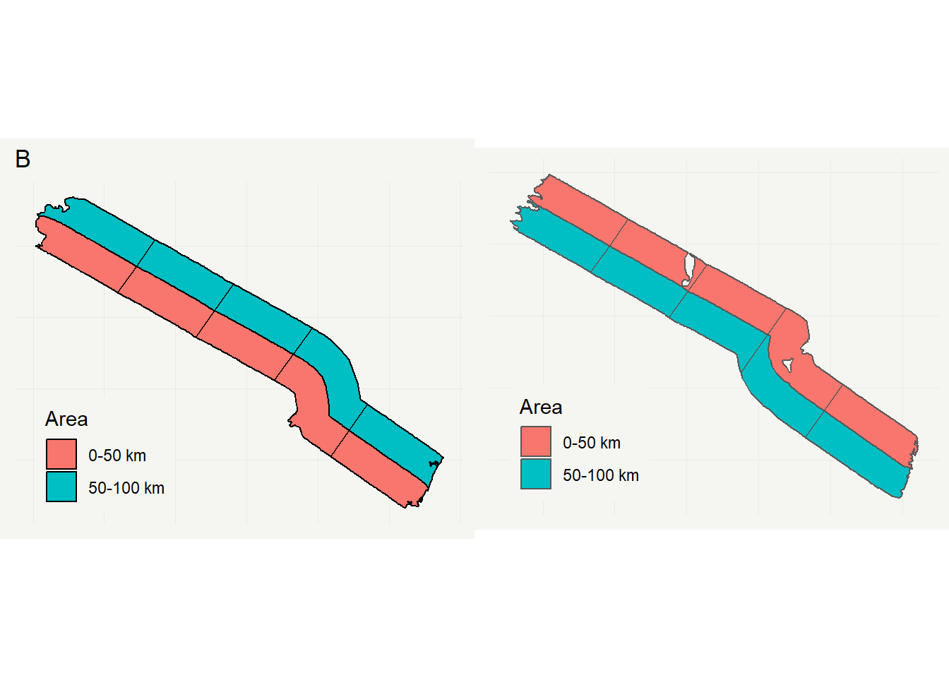 Figure 2.3: Sampling area with sampling bins in Kenya (A) and Nothern Tanzania (B). The red colored areas mark the 0-50 km sampling area and the 50-100 km area is colored in blue.
There are two border areas of interest: the border area between Kenya and Tanzania on the one hand and the border area between Malawi, Tanzania, and Zambia on the other.
Since the border between those states is the defining element for the respective sampling area, they are discussed separately.
The land border between Kenya and Tanzania is the defining element and we can extract it by simply loading the Tanzanian SpatialPolygonsDataFrame, which includes the third administrative division. Waterbodies are declared as such and they are easily removed. In the next step, the SpatialPolygons object is transformed to a SpatialLines object and is cropped by the national borders of Kenya.3 There is a 1 meter buffer around Kenya to make sure it overlaps with the SpatialLines object. The most Western and Eastern points of the border are selected which we will need for the constructions of the bin.
# load polygons
shared_border1_with_kenya <- tanzania_adm3

# remove water bodies and unify Polygons
shared_border_with_kenya <-
  shared_border1_with_kenya[shared_border1_with_kenya$TYPE_3!='Water body',] %>%
  gUnaryUnion


border_tanz_ken <- shared_border_with_kenya %>%
  as("SpatialLines") %>% # transform to SpatialLines
  crop(buffer_shape(kenya_adm0,0.001)[[2]]) # crop by Kenya

# select coordinates of border
border_tanz_ken_geom <- geom(border_tanz_ken) %>%
    as.data.frame %>%
    dplyr::select(x,y)

# select most Western and Eastern point. Here: start and end point of line
start_end <- border_tanz_ken_geom[c(1,nrow(border_tanz_ken_geom)),]
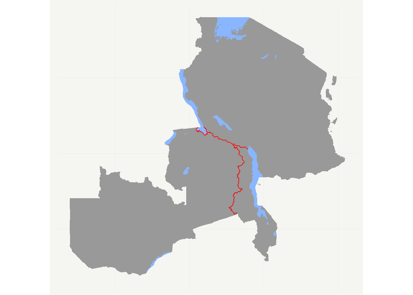 Figure 2.4: Malawi, Tanzania, and Zambia and their common border in red.
The border between Kenya and Tanzania is the start point for building the sampling areas. In our project we want to stratify by a 0-50 and a 50-100 km border area (Figure 2.3 Panel A). Both areas are successively built by implementing the function prepare_sampling_area. The 50-100 km area is constructed in a way that it overlaps with the 0-50 km area and then is cut in the following step. This way we make sure that we do not have any empty space between those two areas.
Finally, we pass both areas in the prepare_sampling_bins function, which further divides both areas in 5 more or less equally sized bins which will serve as the secondary sampling unit. Here, the variable start_end comes in handy because a simple line is drawn to connect both points and the split it into 5 equally sized areas.
The procedure is the same for the Nothern Tanzanian side (Figure 2.3 Panel B).
# KENYA
# 0 - 50 km area
kenya_border_area_0_to_50 <-
  prepare_sampling_area(
    adm0 = kenya_adm0,
    border_spatialline = border_tanz_ken,
    lakes = lakes,
    width_in_km = 50)

# 0 - 50 km area
kenya_border_area_50_to_100 <-
  prepare_sampling_area(
    adm0 = kenya_adm0,
    border_spatialline = border_tanz_ken,
    lakes = lakes,
    width_in_km = 100,
    split_width = 49) %>%
  gDifference(kenya_border_area_0_to_50)

kenya_sampling_bins <-
  prepare_sampling_bins(
    a = kenya_border_area_0_to_50,
    b = kenya_border_area_50_to_100,
    start_end = start_end,
    number_of_bins = 5)

# TANZANIA
# 0 - 50 km area
northern_tanzania_border_area_0_to_50 <- prepare_sampling_area(
  tanzania_adm0,
  border_tanz_ken,
  lakes,
  width_in_km = 50)

# 0 - 50 km area
northern_tanzania_border_area_50_to_100 <- prepare_sampling_area(
  tanzania_adm0,
  border_tanz_ken,
  lakes,
  width_in_km = 100,
  split_width = 49) %>%
  gDifference(northern_tanzania_border_area_0_to_50)

northern_tanzania_sampling_bins <- prepare_sampling_bins(
  a = northern_tanzania_border_area_0_to_50,
  b = northern_tanzania_border_area_50_to_100,
  start_end = start_end,
  number_of_bins = 5)
For the area on the Tanzania side of the Kenya-Tanzania border, the above code is analogous and only the adm0 argument of prepare_sampling_area needs to be changed. Figure 2.3 Panel B shows the resulting sampling area.
2.3 Malawi-Tanzania-Zambia border
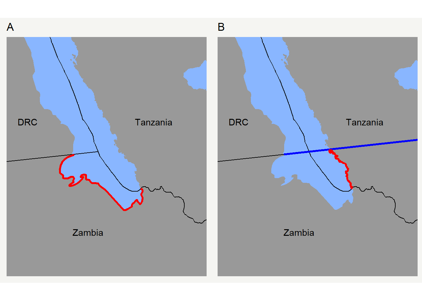 Figure 2.5: Sampling line at lake Tanganyika for Zambia (A) and Tanzania (B). The blue line indicates the prolonged DRC-Zambian border to limit the sampling line on the Tanzanian side of Lake Tanganyika.
The approach for the whole Southern border situation is a bit more complicated since there are no natural cut-off points such as the sea for the Northern border area. Furthermore, the shore of lake Tanganyika in the Western border area between Tanzania and Zambia is part of the line that will be used to draw the sampling area. On the Zambian side, the sampling line stops at the point where Zambia shares a border with the Democratic Republic of the Congo (DRC). The cut-off for the sampling line on the Tanzanian side is determined by the prolonged border line between the DRC and Zambia.
# extract the border that Tanzania shares with Zambia and Malawi
shared_border1_of_tanz <- tanzania_adm3

shared_border_of_tanz2 <- shared_border1_of_tanz[shared_border1_of_tanz$TYPE_3!='Water body',]

shared_border_of_tanz <- gUnaryUnion(shared_border_of_tanz2)

border_for_tanz <- bind(zambia_adm0,malawi_adm0)

# identify lake Tanganyika
tanganyika_full <- lakes[grep("Tanganyika",lakes$name_en),]

# Zambian side
tanganyika_zambia <- border_for_tanz %>%
  as("SpatialLines") %>%
  crop(buffer_shape(tanganyika_full,0.1)[[2]])

# need to prolong border from Zambia
zam_line_to_lake <- tanganyika_zambia@lines[[1]]@Lines[[1]]@coords[1:2,] %>%
  as.data.frame()

split_line_tanzania_tangayika<-
  rbind(new_line_thru_math(lm(y~x,data=zam_line_to_lake)$coef,
                           x_vector = 40,
                           p4s = proj4string(tanganyika_zambia)
  )@lines[[1]]@Lines[[1]]@coords,
  zam_line_to_lake) %>%
  coords_to_line(p4s = proj4string(tanganyika_zambia))

# shore line tangayika tanzani
tanganyika_tanzania<-crop(tanzania_adm0 %>%
                             as("SpatialLines"),
                           buffer_shape(tanganyika_full,10)[[2]])

# coordinates of the intersection between the prolonged border line and the Tanganyika shore
tanganyika_tanzania_split_point <-
  gIntersection(tanganyika_tanzania,split_line_tanzania_tangayika)@coords

# clip tanganyika_tanzania at tanganyika_tanzania_split_point
line_list<-lapply(1:length(tanganyika_tanzania@lines[[1]]@Lines),function(x) {
  l1<-tanganyika_tanzania@lines[[1]]@Lines[[x]]@coords %>%
  as.data.frame() %>%
  filter(y<=tanganyika_tanzania_split_point[1,2])
  if (nrow(l1)==0) return()
  list(coords_to_line(l1,proj4string(tanganyika_zambia)))
})

# Sampling line for the Tanganyika line on the Tanzanian side
tan_line_to_lake<-from_list_to_poly3(line_list) %>%
  crop(tanzania_adm0a) %>%
  gDifference(buffer_shape(zambia_adm0a,0.01)[[2]])
The rest of the sampling line is extracted by defining one end at where the border between Malawi, Tanzania, and the shore of lake Malawi meet and the other where Malawi, Zambia, and Mozambique cross.
# Zambia
border_for_zamb1 <- shared_border_of_tanz %>%
  as("SpatialLines") %>%
  crop(buffer_shape(zambia_adm0,0.001)[[2]])

border_for_zamb2 <- bind(border_for_zamb1,tanganyika_zambia,maw_zam)

# Tanzania
border_for_tanz_line1 <- border_for_tanz %>%
  as("SpatialLines")

border_for_tanz_line2 <- crop(border_for_tanz_line1,
                              buffer_shape(tanzania_adm0,0.001)[[2]])

border_for_tanz3 <- bind(tan_line_to_lake,border_for_tanz_line2)

# Malawi
border_for_maw1 <- shared_border_of_tanz %>%
  as("SpatialLines") %>%
  crop(buffer_shape(malawi_adm0,0.001)[[2]])

border_for_maw2 <- list(border_for_maw1,maw_zam) %>%
  do.call(bind,.)
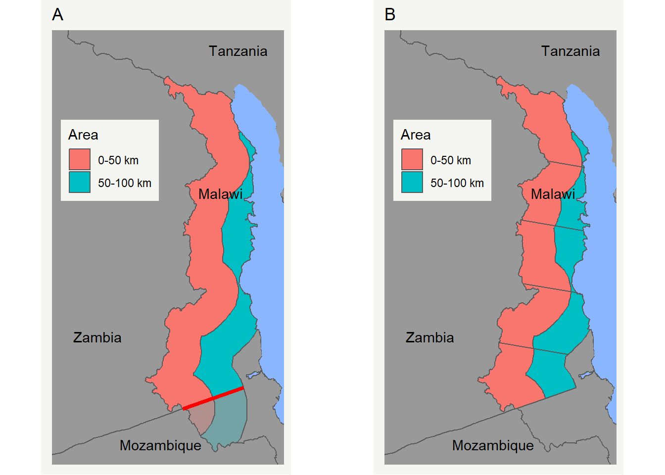 Figure 2.6: Sampling areas in Malawi. Panel A shows the cut-off facilitated by the extended Zambian border line (red) and Panel B shows the final sampling area which is divided in ten bins.
2.3.1 Malawi
Since the project is only interested in border areas between the three countries, the buffered area for Malawi gets clipped were it extends to the Mozambican border. Similar to the cut-off at the Tanzanian border for the sampling line, the Zambian border is extended and used to clip the sampling area in Malawi. Panel A in Figure 2.6 shows the prolonged Zambian border line in red and the area. The part that is cut-off by the prolonged border is marked by lower saturation. Panel B shows the final sampling area for Malawi.
## create cut off line for malawi
rest_zam1 <- gDifference(zambia_adm0 %>%
                           as("SpatialLines"),
                         border_for_maw2) %>%
  gDifference(border_for_tanz3)

rest_zam2 <- rest_zam1@lines[[1]]@Lines[[1]]@coords  %>%
  as.data.frame

rest_zam3 <- rest_zam2 %>%
  mutate(x_max=max(x)) %>%
  filter(x!=x_max) %>%
  mutate(x_max2=max(x)) %>%
  filter(x==x_max2) %>%
  dplyr::select(x_max,x_max2) %>%
  unlist

rest_zam4 <- rest_zam2 %>%
  filter(x%in%rest_zam3)


split_line_malawi <- rbind(
  c(20,lm(y~x,rest_zam4)$coef[2]*20+lm(y~x,rest_zam4)$coef[1]),
  rest_zam4,
  c(40,lm(y~x,rest_zam4)$coef[2]*40+lm(y~x,rest_zam4)$coef[1])
) %>%
  coords_to_line(proj4string(rest_zam1))

coords1_maw <- split_line_malawi@lines[[1]]@Lines[[1]]@coords %>%
  as.data.frame()

coords2_maw <- coords1_maw %>%
  mutate(y=y+10)

cropper_maw <- rbind(coords1_maw,coords2_maw[3:1,]) %>%
  Polygon %>%
  list %>%
  Polygons(ID=1) %>%
  list %>%
  SpatialPolygons(proj4string =
                    CRS(proj4string(split_line_malawi)))


# malawi border area
maw_border_area_0_to_50 <- prepare_sampling_area(
  malawi_adm0,border_for_maw2,lakes,width_in_km = 50)

maw_border_area_0_to_50_cropped <- crop(maw_border_area_0_to_50,
                                      cropper_maw)

maw_border_area_50_to_100 <- prepare_sampling_area(
  malawi_adm0,border_for_maw2,lakes,width_in_km = 100,split_width = 49) %>%
  gDifference(maw_border_area_0_to_50)

maw_border_area_50_to_100_cropped <- crop(maw_border_area_50_to_100,
                                      cropper_maw)
# Malawi bins
# preparing for border_for_maw3
border_for_maw3 <- lapply(1:length(border_for_maw2),function(x) {
r1<-gLineMerge(border_for_maw2[x,])
r1<-r1@lines[[1]]@Lines[[1]]@coords
r1[nrow(r1):1,] %>% coords_to_line(proj4string(border_for_maw2))
}) %>%
do.call(rbind,.)
maw_start_end <- lapply(1:length(border_for_maw3),function(x) {
border_for_maw3_geom<-geom(border_for_maw3[x,])
border_for_maw3_geom[c(1,nrow(border_for_maw3_geom)),c("x","y")]
}) %>%
do.call(rbind,.) %>%
as.data.frame
maw_sampling_bin <- prepare_sampling_bins(
a = maw_border_area_0_to_50,
b = maw_border_area_50_to_100,
start_end = maw_start_end[c(2,4),],
number_of_bins = 5)2.3.2 Tanzania Southern border area
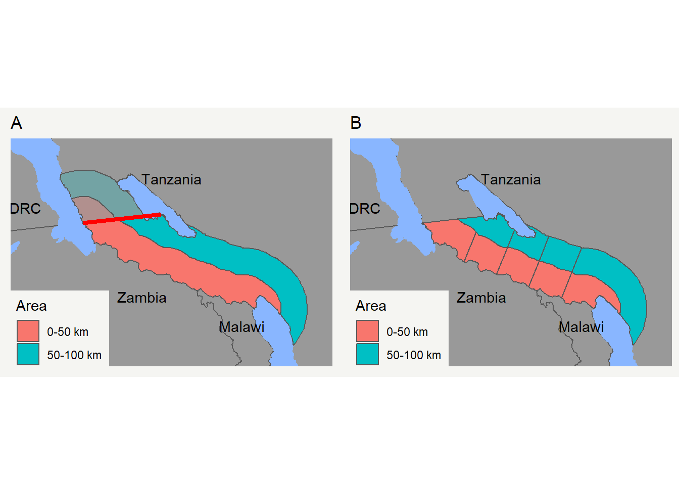 Figure 2.7: Southern border area of Tanzania. Panel A shows the cut-off facilitated by the prolonged Zambian border line (red). Panel B shows the final sampling area which is divided in 9 bins, because the most Western 50-100 km bins were merged due to the small size of one of them.
The Southern border area of Tanzania is also cutted off. In general, the lake sides might provide interesting variation, however this is not true if the country on the opposite shore does not belong to the countries under investigation. Hence, the prolonged Zambian border line is used to clipp the buffer zone (Figure 2.7 Panel A). Note that the two most Western 50-100 km bins were merged, because of the small size of one of them (Panel B).
coords1 <- split_line_tanzania_tangayika@lines[[1]]@Lines[[1]]@coords %>%
  as.data.frame()

coords2 <- coords1 %>%
  mutate(y=y-10)

cropper_tanz <- rbind(coords1,coords2[3:1,]) %>%
  polygon_from_coords(proj4string(split_line_tanzania_tangayika)) %>%
  buffer_shape(0)

cropper_tanz<-cropper_tanz[[2]]

# 0 to 50
southern_tanzania_border_area_0_to_50 <- prepare_sampling_area(
  tanzania_adm0,border_for_tanz3,lakes,
  width_in_km = 50)

southern_tanzania_border_area_50_to_100 <- prepare_sampling_area(
  tanzania_adm0,border_for_tanz3,lakes,
  width_in_km = 100,split_width = 49) %>%
  gDifference(southern_tanzania_border_area_0_to_50)

southern_tanzania_border_area_0_to_50_cropped <-
  crop(southern_tanzania_border_area_0_to_50,cropper_tanz)

southern_tanzania_border_area_50_to_100_cropped <-
  crop(southern_tanzania_border_area_50_to_100,cropper_tanz)


# preparing border_for_tanz4
border_for_tanz4 <- rbind(border_for_tanz3[1,],gLineMerge(border_for_tanz3[2,]))

points_from_tanzania_border <- geom(border_for_tanz4) %>%
  as.data.frame() %>%
  dplyr::select(x,y)

points_from_tanzania_border_start_end <-
  points_from_tanzania_border[c(1,nrow(points_from_tanzania_border)),]

# sampling bins
southern_tanzania_sampling_bins1 <- prepare_sampling_bins(
  a=southern_tanzania_border_area_0_to_50_cropped,
  b=southern_tanzania_border_area_50_to_100_cropped,
  start_end = points_from_tanzania_border_start_end,
  number_of_bins = 5)

# merge the two Western most 50-100km bins
southern_tanzania_sampling_bins <- bind(tanzania_sampling_bins1[c(1:5,8:10),],
                               gUnaryUnion(tanzania_sampling_bins1[6:7,]))
2.3.3 Zambia
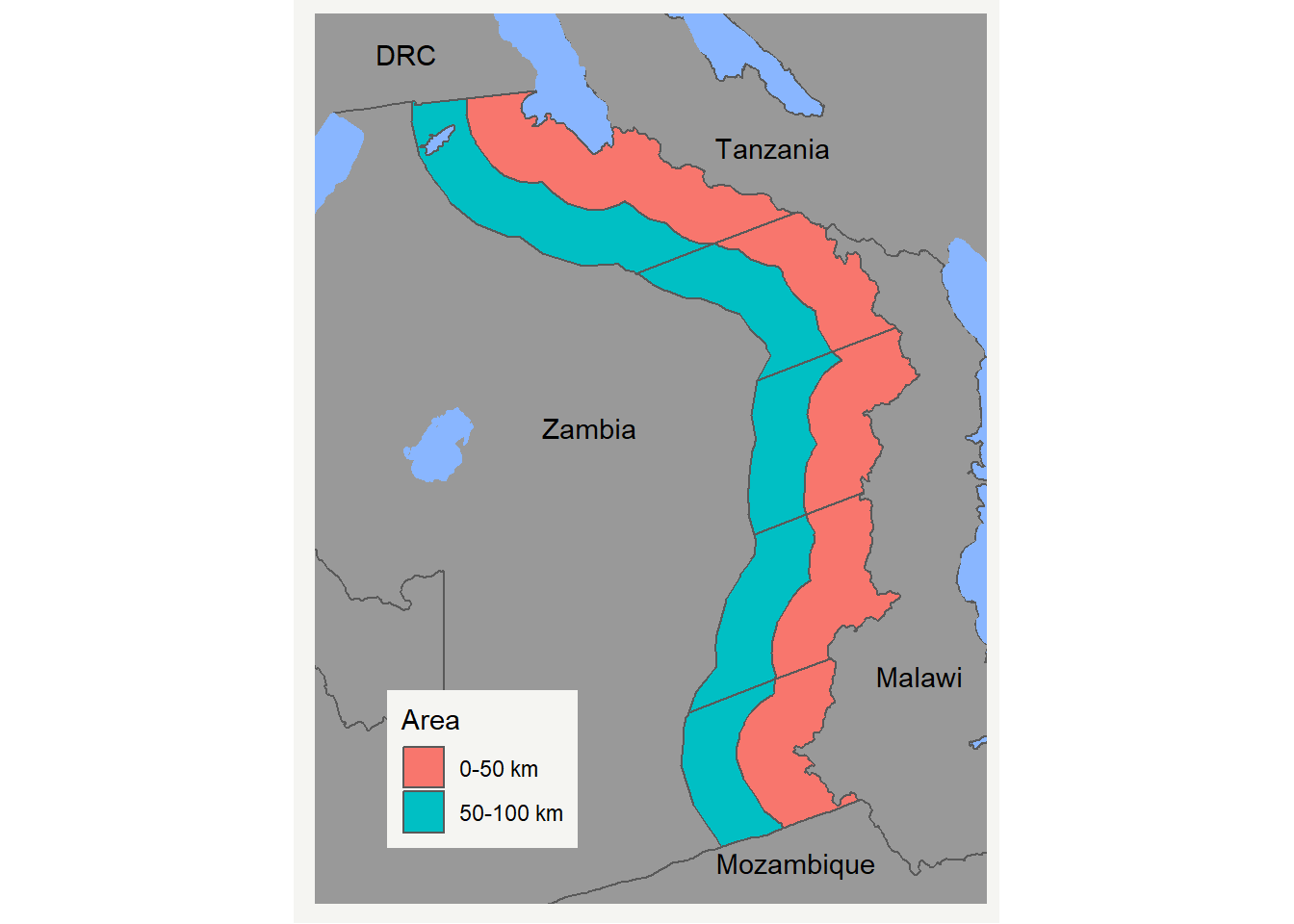 Figure 2.8: Sampling area in Zambia.
The Zambian sampling area does not need any further cutting or merging since it determined the cut-off lines for the Malawian and Southern Tanzanian sampling area (Figure 2.8).
zam_border_area_0_to_50 <- prepare_sampling_area(
  zambia_adm0,border_for_zamb2,lakes,width_in_km = 50)

# 50 to 100
zam_border_area_50_to_100 <- prepare_sampling_area(
  zambia_adm0,border_for_zamb2,lakes,width_in_km = 100,
  split_width = 49) %>%
  gDifference(zam_border_area_0_to_50)


# take right points for the border
border_for_zamb3 <- lapply(1:length(border_for_zamb2),function(x) {
  gLineMerge(border_for_zamb2[x,])
}) %>%
  do.call(rbind,.)

border_for_zamb3_geom <- geom(border_for_zamb3) %>%
  as.data.frame %>%
  dplyr::select(x,y)


zam_start_end <- lapply(1:length(border_for_zamb3),function(x) {
  border_for_zamb3_geom<-geom(border_for_zamb3[x,])
  border_for_zamb3_geom[c(1,nrow(border_for_zamb3_geom)),c("x","y")]
}) %>%
  do.call(rbind,.) %>%
  as.data.frame


zambia_sampling_bin <- prepare_sampling_bins(a = zam_border_area_0_to_50,
                                             b = zam_border_area_50_to_100,
                                             start_end = zam_start_end[4:5,],
                                             number_of_bins = 5)
2.4 Summarising: Sampling border areas
leaflet() %>%
  addProviderTiles(providers$Esri.NatGeoWorldMap) %>%
  addPolygons(data=southern_tanzania_sampling_bins) %>%
  addPolygons(data=northern_tanzania_sampling_bins) %>%
  addPolygons(data=kenya_sampling_bins) %>%
  addPolygons(data=maw_sampling_bin) %>%
  addPolygons(data=zambia_sampling_bin) %>%
  addPolygons(data=dar_bins_6) %>%
  addPolygons(data=nairobi_bins) %>%
  addPolygons(data=lusaka_bins)
Figure 2.9: Sampling border areas in the four countries.