Chapter 2 Spatial polygon areas

First, I will discuss the urban sampling areas before turning to the more complicated border areas.

2.1 Cities

The sampling area is defined by taking a 50 km radius around the center of the respective city. The coordinates from Table 2.1 are taken from Wikipedia.11 https://Wikipedia.org

Table 2.1: Longitude and latitude of Lilongwe, Lusaka, and Nairobi.

City	Longitude	Latitude
Lilongwe	33.783333	-13.983333
Lusaka	28.283333	-15.416667
Nairobi	36.81667	-1.28333

The geosampling::prepare_sampling_bins_city function draws two circles around a point and splits both circles along the horizontal and the vertical axis in 8 pieces.
The function takes in the arguments adm0 for a variable of class SpatialPolygons, which contains the national border of the respective country, the coordinates of the respective city (coords), a variable of class SpatialPolygons, which contains lakes, and radius_inner_circle and radius_outer_circle to determine the radius of both circles.

lusaka_bins <- prepare_sampling_bins_city(
  adm0 = zambia_adm0,
  coords=city_table[2,2:3],
  lakes = lakes,
  radius_inner_circle=25,
  radius_outer_circle=50)

Figure ?? shows the sampling areas for Dar Es Salaam. In Panel A Dar es Salaam has 7 different sampling areas, but one is rather small and is merged with its neighboring area (B and C).22 Map style borrowed from Timo Grossenbacher.
The sampling areas for all three cities are visualized in Figure 2.4.

2.2 Malawi-Zambia border

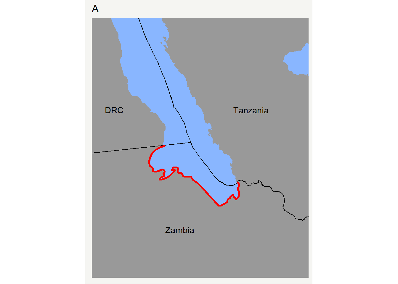$Sampling line at lake Tanganyika for Zambia. \label{fig:zambiaztanganyikashore}$ Figure 2.1: Sampling line at lake Tanganyika for Zambia.

The approach for the whole Southern border situation is a bit more complicated since there are no natural cut-off points such as the sea for the Northern border area. Furthermore, the shore of lake Tanganyika in the Western border area between Tanzania and Zambia is part of the line that will be used to draw the sampling area. On the Zambian side, the sampling line stops at the point where Zambia shares a border with the Democratic Republic of the Congo (DRC). The cut-off for the sampling line on the Tanzanian side is determined by the prolonged border line between the DRC and Zambia.

# extract the border that Tanzania shares with Zambia and Malawi
shared_border1_of_tanz <- tanzania_adm3

shared_border_of_tanz2 <- shared_border1_of_tanz[shared_border1_of_tanz$TYPE_3!='Water body',]

shared_border_of_tanz <- gUnaryUnion(shared_border_of_tanz2)

border_for_tanz <- bind(zambia_adm0,malawi_adm0)

# identify lake Tanganyika
tanganyika_full <- lakes[grep("Tanganyika",lakes$name_en),]

# Zambian side
tanganyika_zambia <- border_for_tanz %>% 
  as("SpatialLines") %>% 
  crop(buffer_shape(tanganyika_full,0.1)[[2]])

# need to prolong border from Zambia
zam_line_to_lake <- tanganyika_zambia@lines[[1]]@Lines[[1]]@coords[1:2,] %>% 
  as.data.frame()

split_line_tanzania_tangayika<-
  rbind(new_line_thru_math(lm(y~x,data=zam_line_to_lake)$coef,
                           x_vector = 40,
                           p4s = proj4string(tanganyika_zambia)
  )@lines[[1]]@Lines[[1]]@coords,
  zam_line_to_lake) %>% 
  coords_to_line(p4s = proj4string(tanganyika_zambia)) 

# shore line tangayika tanzani
tanganyika_tanzania<-crop(tanzania_adm0 %>% 
                             as("SpatialLines"),
                           buffer_shape(tanganyika_full,10)[[2]])

# coordinates of the intersection between the prolonged border line and the Tanganyika shore
tanganyika_tanzania_split_point <- 
  gIntersection(tanganyika_tanzania,split_line_tanzania_tangayika)@coords

# clip tanganyika_tanzania at tanganyika_tanzania_split_point
line_list<-lapply(1:length(tanganyika_tanzania@lines[[1]]@Lines),function(x) {
  l1<-tanganyika_tanzania@lines[[1]]@Lines[[x]]@coords %>% 
  as.data.frame() %>%
  filter(y<=tanganyika_tanzania_split_point[1,2]) 
  if (nrow(l1)==0) return()
  list(coords_to_line(l1,proj4string(tanganyika_zambia)))
})

# Sampling line for the Tanganyika line on the Tanzanian side
tan_line_to_lake<-from_list_to_poly3(line_list) %>%  
  crop(tanzania_adm0a) %>% 
  gDifference(buffer_shape(zambia_adm0a,0.01)[[2]])

For Zambian, the sampling area extends to all areas that are adjunct to the Tanzanian and Malawian border. The border line starts in the West as the shore of the Tanganyika lake ().
The rest of the sampling line is extracted by defining one end at where the border between Malawi, Tanzania, and the shore of lake Malawi meet and the other where Malawi, Zambia, and Mozambique cross.

# Zambia
border_for_zamb1 <- shared_border_of_tanz %>% 
  as("SpatialLines") %>% 
  crop(buffer_shape(zambia_adm0,0.001)[[2]])

border_for_zamb2 <- bind(border_for_zamb1,tanganyika_zambia,maw_zam) 

# Tanzania
border_for_tanz_line1 <- border_for_tanz %>% 
  as("SpatialLines")

border_for_tanz_line2 <- crop(border_for_tanz_line1,
                              buffer_shape(tanzania_adm0,0.001)[[2]])

border_for_tanz3 <- bind(tan_line_to_lake,border_for_tanz_line2)

# Malawi
border_for_maw1 <- shared_border_of_tanz %>% 
  as("SpatialLines") %>% 
  crop(buffer_shape(malawi_adm0,0.001)[[2]])

border_for_maw2 <- list(border_for_maw1,maw_zam) %>% 
  do.call(bind,.)

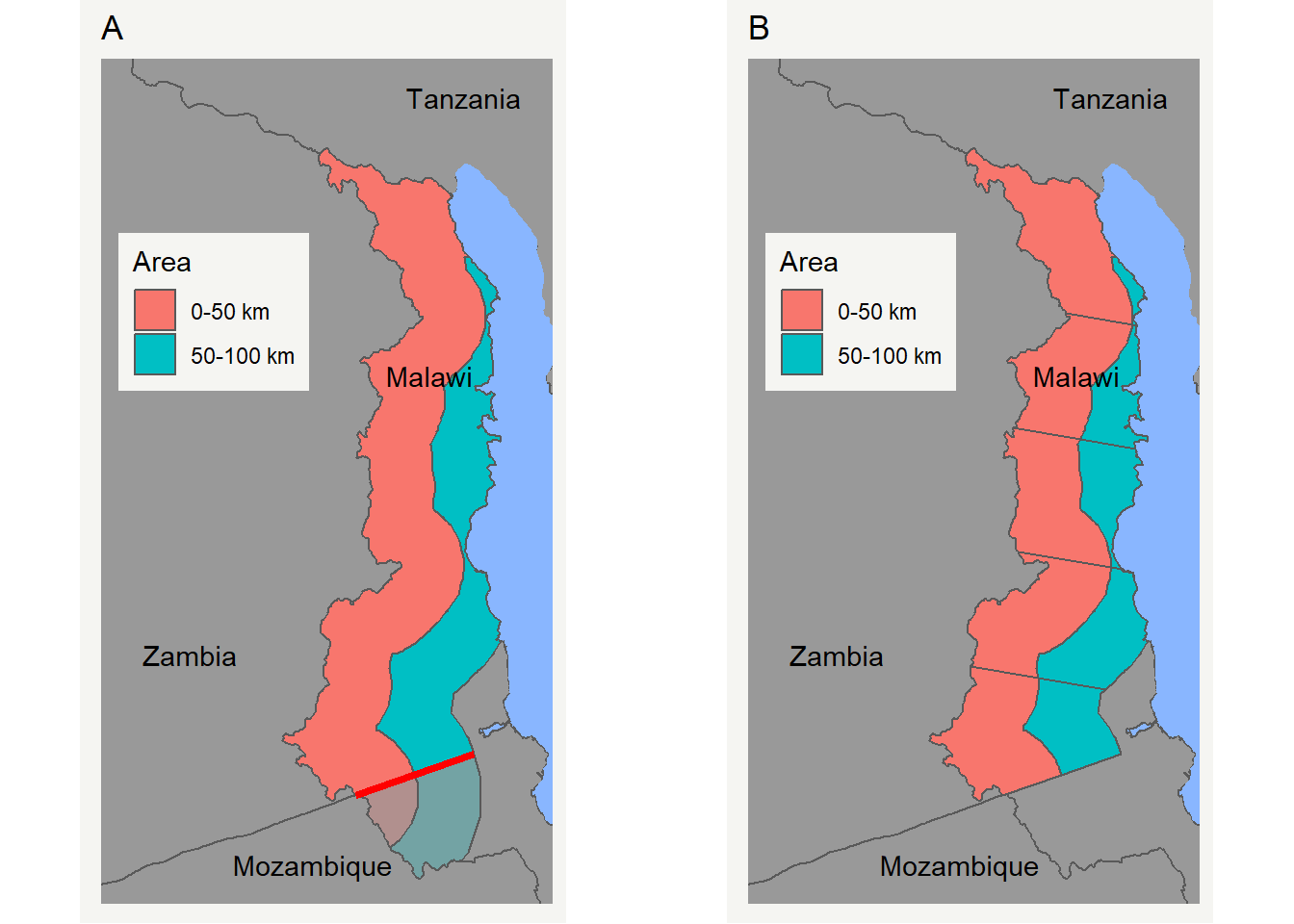Figure 2.2: Sampling areas in Malawi. Panel A shows the cut-off facilitated by the extended Zambian border line (red) and Panel B shows the final sampling area which is divided in ten bins.

2.2.1 Malawi

Since the project is only interested in border areas between the three countries, the buffered area for Malawi gets clipped were it extends to the Mozambican border. Similar to the cut-off at the Tanzanian border for the sampling line, the Zambian border is extended and used to clip the sampling area in Malawi. Panel A in Figure 2.2 shows the prolonged Zambian border line in red and the area. The part that is cut-off by the prolonged border is marked by lower saturation. Panel B shows the final sampling area for Malawi.

## create cut off line for malawi
rest_zam1 <- gDifference(zambia_adm0 %>% 
                           as("SpatialLines"),
                         border_for_maw2) %>% 
  gDifference(border_for_tanz3)

rest_zam2 <- rest_zam1@lines[[1]]@Lines[[1]]@coords  %>% 
  as.data.frame

rest_zam3 <- rest_zam2 %>%
  mutate(x_max=max(x)) %>% 
  filter(x!=x_max) %>% 
  mutate(x_max2=max(x)) %>% 
  filter(x==x_max2) %>% 
  dplyr::select(x_max,x_max2) %>% 
  unlist

rest_zam4 <- rest_zam2 %>% 
  filter(x%in%rest_zam3)


split_line_malawi <- rbind(
  c(20,lm(y~x,rest_zam4)$coef[2]*20+lm(y~x,rest_zam4)$coef[1]),
  rest_zam4,
  c(40,lm(y~x,rest_zam4)$coef[2]*40+lm(y~x,rest_zam4)$coef[1])
) %>% 
  coords_to_line(proj4string(rest_zam1))

coords1_maw <- split_line_malawi@lines[[1]]@Lines[[1]]@coords %>% 
  as.data.frame()

coords2_maw <- coords1_maw %>% 
  mutate(y=y+10)

cropper_maw <- rbind(coords1_maw,coords2_maw[3:1,]) %>% 
  Polygon %>% 
  list %>%
  Polygons(ID=1) %>% 
  list %>% 
  SpatialPolygons(proj4string = 
                    CRS(proj4string(split_line_malawi)))


# malawi border area
maw_border_area_0_to_50 <- prepare_sampling_area(
  malawi_adm0,border_for_maw2,lakes,width_in_km = 50)

maw_border_area_0_to_50_cropped <- crop(maw_border_area_0_to_50,
                                      cropper_maw)

maw_border_area_50_to_100 <- prepare_sampling_area(
  malawi_adm0,border_for_maw2,lakes,width_in_km = 100,split_width = 49) %>% 
  gDifference(maw_border_area_0_to_50)

maw_border_area_50_to_100_cropped <- crop(maw_border_area_50_to_100,
                                      cropper_maw)

# Malawi bins
# preparing for border_for_maw3
border_for_maw3 <- lapply(1:length(border_for_maw2),function(x) {
  r1<-gLineMerge(border_for_maw2[x,])
  r1<-r1@lines[[1]]@Lines[[1]]@coords
  r1[nrow(r1):1,] %>% coords_to_line(proj4string(border_for_maw2))
}) %>% 
  do.call(rbind,.)

maw_start_end <- lapply(1:length(border_for_maw3),function(x) {
  border_for_maw3_geom<-geom(border_for_maw3[x,])
  border_for_maw3_geom[c(1,nrow(border_for_maw3_geom)),c("x","y")]
}) %>% 
  do.call(rbind,.) %>% 
  as.data.frame

maw_sampling_bin <- prepare_sampling_bins(
  a = maw_border_area_0_to_50,
  b = maw_border_area_50_to_100,
  start_end = maw_start_end[c(2,4),],
  number_of_bins = 5)

2.2.1 Tanzania Southern border area

The Southern border area of Tanzania is also cutted off. In general, the lake sides might provide interesting variation, however this is not true if the country on the opposite shore does not belong to the countries under investigation. Hence, the prolonged Zambian border line is used to clipp the buffer zone (Figure ?? Panel A). Note that the two most Western 50-100 km bins were merged, because of the small size of one of them (Panel B).

2.2.2 Zambia

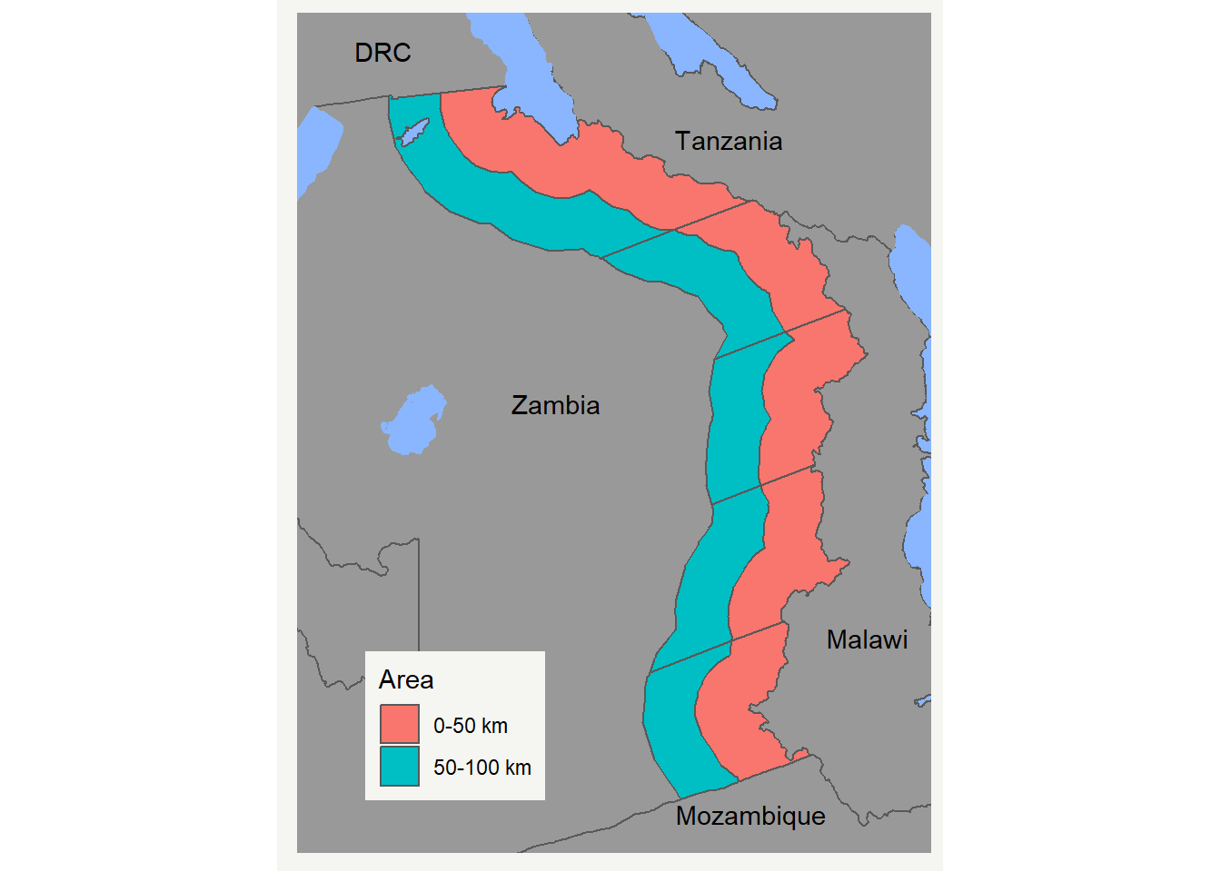Figure 2.3: Sampling area in Zambia.

The Zambian sampling area does not need any further cutting or merging since it determined the cut-off lines for the Malawian and Southern Tanzanian sampling area (Figure 2.3).

zam_border_area_0_to_50 <- prepare_sampling_area(
  zambia_adm0,border_for_zamb2,lakes,width_in_km = 50)

# 50 to 100
zam_border_area_50_to_100 <- prepare_sampling_area(
  zambia_adm0,border_for_zamb2,lakes,width_in_km = 100,
  split_width = 49) %>% 
  gDifference(zam_border_area_0_to_50)


# take right points for the border
border_for_zamb3 <- lapply(1:length(border_for_zamb2),function(x) {
  gLineMerge(border_for_zamb2[x,])
}) %>% 
  do.call(rbind,.)

border_for_zamb3_geom <- geom(border_for_zamb3) %>% 
  as.data.frame %>% 
  dplyr::select(x,y)


zam_start_end <- lapply(1:length(border_for_zamb3),function(x) {
  border_for_zamb3_geom<-geom(border_for_zamb3[x,])
  border_for_zamb3_geom[c(1,nrow(border_for_zamb3_geom)),c("x","y")]
}) %>% 
  do.call(rbind,.) %>% 
  as.data.frame


zambia_sampling_bin <- prepare_sampling_bins(a = zam_border_area_0_to_50,
                                             b = zam_border_area_50_to_100,
                                             start_end = zam_start_end[4:5,],
                                             number_of_bins = 5)

2.3 Summarising: Sampling border areas

leaflet() %>% 
  addProviderTiles(providers$Esri.NatGeoWorldMap) %>% 
  addPolygons(data=maw_sampling_bin) %>% 
  addPolygons(data=zambia_sampling_bin) %>% 
  addPolygons(data=lilongwe_bins) %>% 
  addPolygons(data=nairobi_bins) %>% 
  addPolygons(data=lusaka_bins)

Figure 2.4: Sampling border areas in the four countries.

2.4 Districts likely to be sampled

kenya_districs <- 
  kenya_adm2[over(kenya_adm2,gUnaryUnion(nairobi_bins),
                  returnList = FALSE) %>%  
               is.na() %>% 
               `!` %>% 
               which,] %>% 
  st_as_sf()

zambia_districts <- 
  zambia_adm2[over(zambia_adm2,
                   gUnaryUnion(bind(lusaka_bins,
                                    zambia_sampling_bin))) %>% 
                is.na() %>% 
                `!` %>%
                which,] %>% 
  st_as_sf()


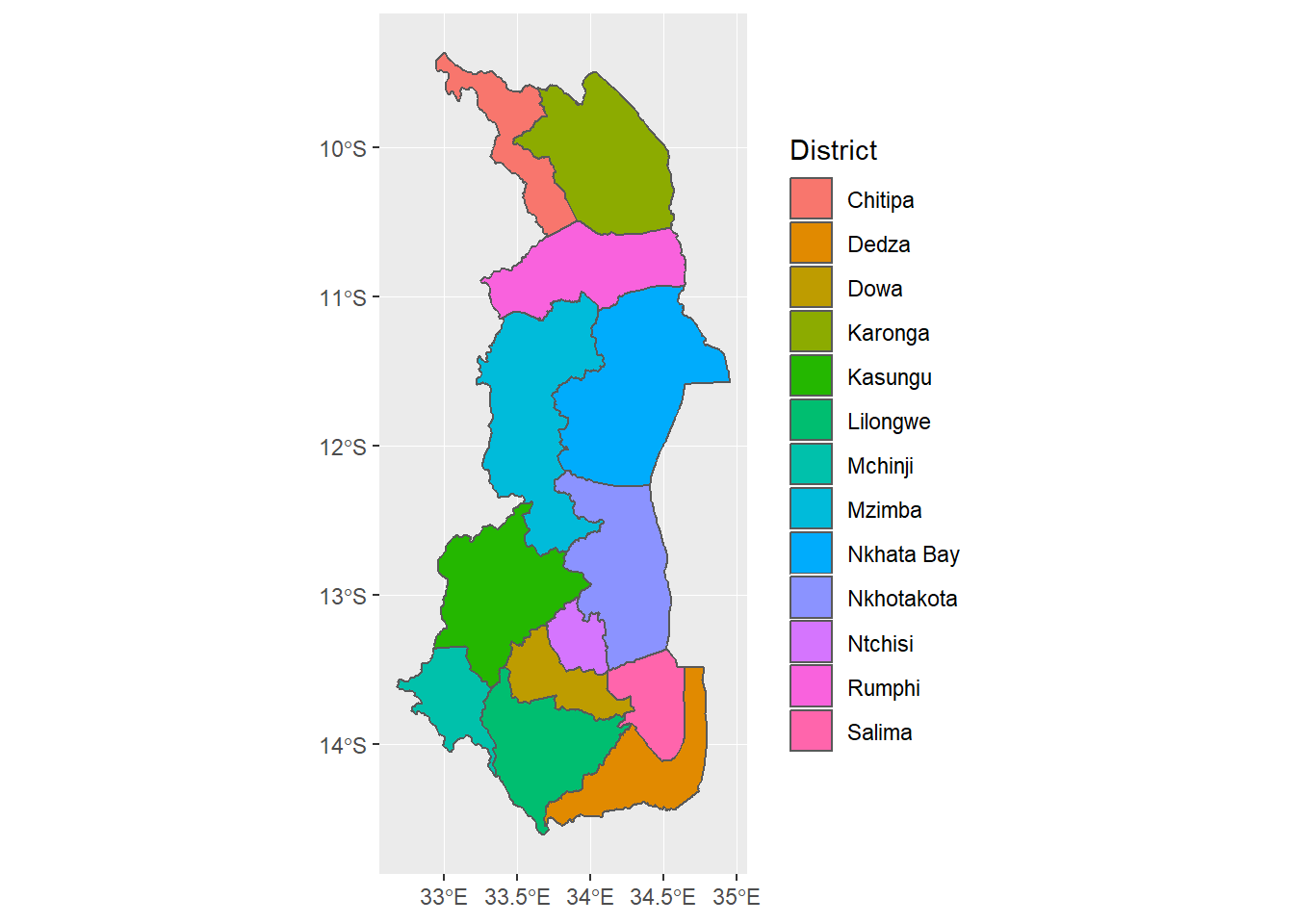
malawi_districs <- malawi_adm1[over(malawi_adm1,
                 gUnaryUnion(bind(lilongwe_bins,maw_sampling_bin))) %>% 
              is.na() %>% 
              `!` %>% 
              which,] %>% 
  st_as_sf()

Figure 2.5: Districts in Kenya

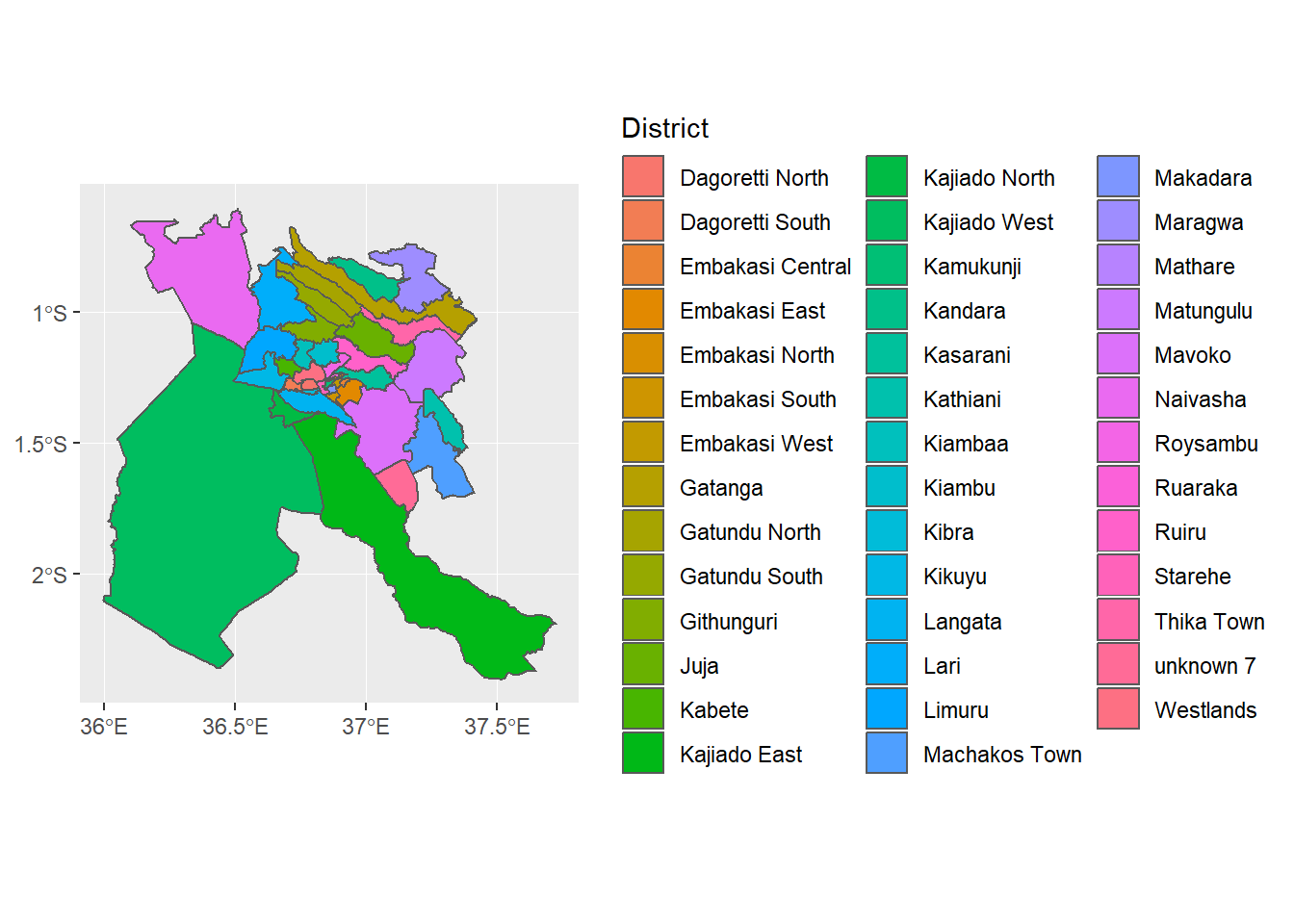
Figure 2.6: Districts in Kenya

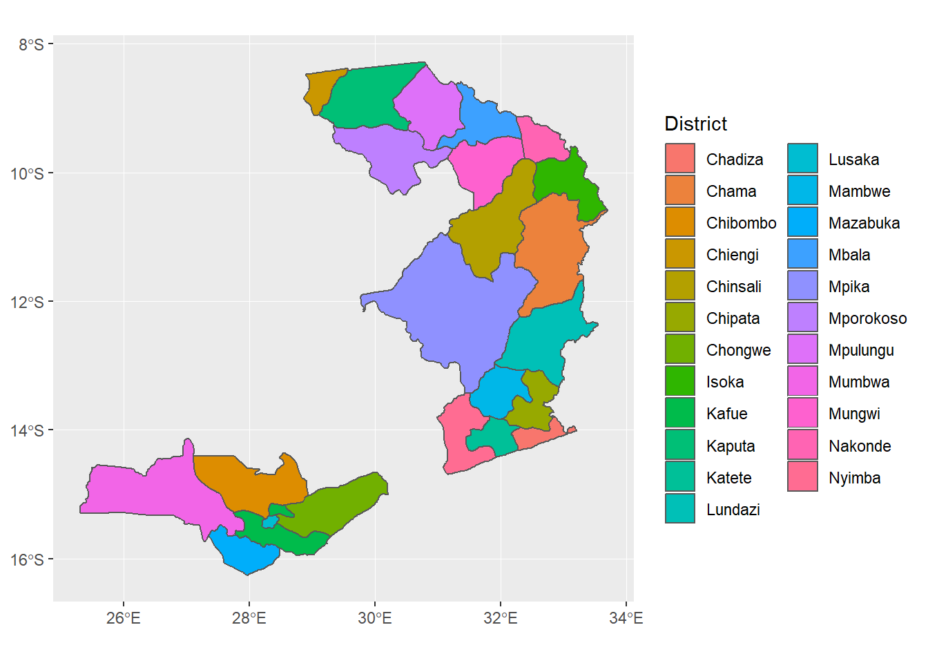
Figure 2.7: Districts in Kenya